Data Collection, Processing & Analysis
On this page:
This section begins with a series of vignettes describing how GP-B data were collected and stored, how safemodes protected the spacecraft, science instruments and data, how anomalies such as computer memory errors were handled, and how intentional telescope dither and stellar aberration were used to calibrate the science data signals received. These vignettes were originally written to answer the question most asked throughout the mission by people around the world who were following GP-B: “Why is it that proton hits to the spacecraft, computer memory errors, and other anomalies and glitches that occurred during the science phase of the mission will have little, if any effect on the final experimental results?” This section ends with an overview of the data analysis process through which we will arrive at the final experimental results.
Data Collection & Telemetry
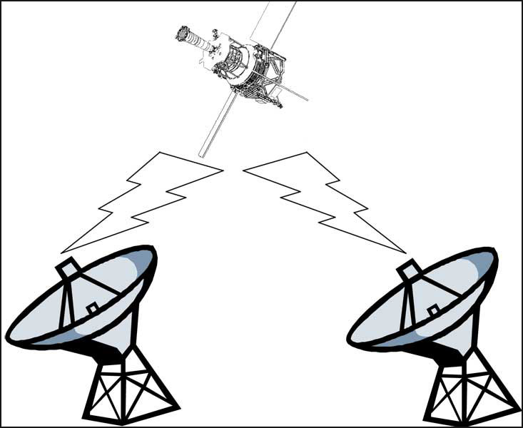
GP-B spacecraft communications
ground link
Our GP-B spacecraft has the capability of autonomously collecting data—in real time—from over 9,000 sensors (aka monitors). Onboard the spacecraft there is memory bank, called a solid-state recorder (SSR), which has the capacity to hold about 15 hours of spacecraft data—both system status data and science data. The spacecraft does not communicate directly with the GP-B Mission Operations Center (MOC) here at Stanford. Rather, it communicates with a network of NASA telemetry satellites, called TDRSS (Tracking and Data Relay Satellite System), and with NASA ground tracking stations.
Many spacecraft share these NASA telemetry facilities, so during the mission, GP-B had to schedule time to communicate with them. These scheduled spacecraft communication sessions are called “passes,” and during the flight mission, the GP-B spacecraft typically completed 6-10 TDRSS passes and 4 ground station passes each day. During these communications passes, commands were relayed to the spacecraft from the MOC, and data were relayed back via the satellites, ground stations, and NASA data processing facilities. The TDRSS links have a relatively slow data rate, so we could only collect spacecraft status data and send commands during TDRSS passes. We were able to collect science data only during the ground passes. That’s the “big picture.” Following is a more detailed look at the various data collection and communication systems described above.
Solid State Recorder
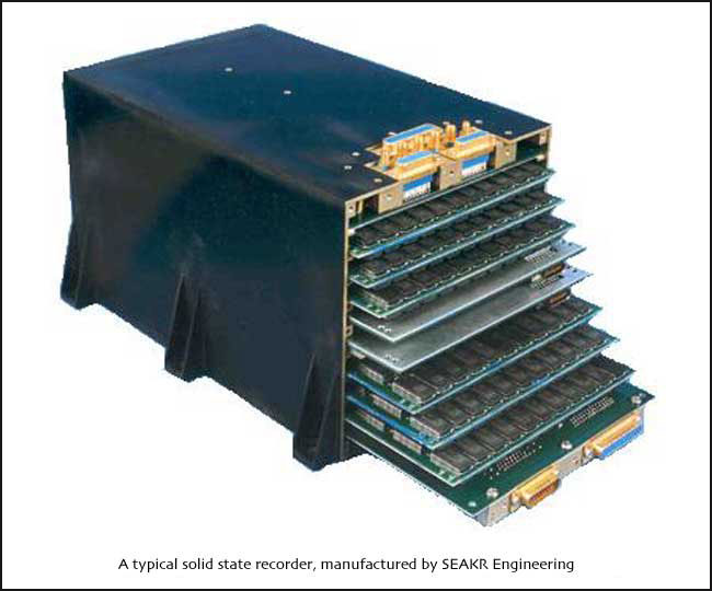
A typical solid state rcorder
An SSR is basically a bank of Random Access Memory (RAM) boards, used on-board spacecraft to collect and store data. It is typically a stand-alone “black box,” containing multiple memory boards and controlling electronics that provides management of data, fault tolerance, and error detection and correction. The SSR onboard the GP-B spacecraft has approximately 185 MB of memory—enough to hold about 15.33 hours of spacecraft data. This is not enough memory to hold all of the data generated by the various monitors, so the GP-B Mission Operations staff controlled what data were collected at any given time, through commands sent to the spacecraft.Many instruments on-board the spacecraft have their own memory banks. Data rates from these instruments vary—most send data every 0.1 second, but some are faster and others slower. The data from all of these instruments are collected by the primary data bus (communication path) and sent to the central computer, called the CCCA. The CCCA then sends the data to the SSR. The data were categorized into five subtypes:
- Sensor programmable telemetry—High data rate of 0.1 seconds, greater than 9000 monitors, mostly used for science & engineering)—this is GP-B’s “primary” useful data, including most science data.
- Event data—For example, whether the vehicle is in eclipse (tells when we entered eclipse behind the earth and when we emerged)
- Database readouts—Used to confirm that the on-board database is the same as the ground folks think it is—e.g., use this to verify that say, filter setting commands, were received and enacted.
- Memory readout (MRO)—Used to ensure that the binary memory on-board is the same (error free) memory we think it is—this is where single & multi-bit errors occur (this is not collected data, but only programmable processes—i.e., the spacecraft’s Operating System). If we find errors in the MROs, we can re-load the memory. Solar wind (proton hits), for example, can cause errors here.
- Snapshot data—This is extremely high-speed data (1/200th of a second) from the SQUID (Super- Conducting Quantum Interference Device), Telescope and Gyro readout systems.The CCCA does some on-board data reduction, performing Fast Fourier Transforms (FFT) on some of the incoming SRE data. This on-board reduction is necessary, because we do not have room in our SSR, nor the telemetry bandwidth, to relay the high-rate data back to the MOC all the time. (Perhaps we should upgrade to DSL…) However, like all numerical analysis methodology, an FFT can become “lost” because an FFT is not always performed from the same starting abscissa (x-axis) value. The Snapshot allows us to see some of the original data sets being used for the FFTs and confirm that they are not los—or if they are, we can fix them by making a programmed adjustment on-board. Other systems—the Telescope Readout (TRE) and Gyro Suspension System (GSS)—use their snapshots for similar instrumentation and data reduction validity checks.
Data were stored to the SSR in a “First in, First out” queue. Once the memory is 15.33 hours full, the new data begins to overwrite the oldest data collected. That’s why it was a good idea to dump the SSR to the ground at least every 12 –15 hours (for safety!), which is exactly what we did.
Telemetry—TDRSS & Ground Stations
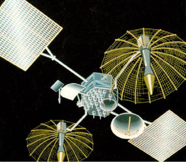
Drawing of a NASA TDRSS satellite
So, how did we talk to the spacecraft and retrieve our data? NASA communicates with its spacecraft in several ways. Its highest availability is through TDRSS, two communications satellites in orbit, just waiting for communications. These two satellites can’t handle much data at a time, and we could transmit to them only at a 1K or 2K (kilobit per second) rate. For GP-B, this rate is only fast enough to exchange status information and commands; it was not fast enough for downloading science data.
NASA also uses ground-based stations. There are several around the world, but each ground station network used is determined by satellite type and orbit. Because GP-B is in a polar orbit communicating primarily at 32K (32kilobits per second), we used the NASA Goddard “Ground Network.” This network includes stations in Poker Flats, Alaska, Wallops, Virginia, Svalbard, Norway, and McMurdo station, Antarctica. Communication with the South Pole station was not as reliable as the others, but we did use the McMurdo ground station on a few occasions during the mission.
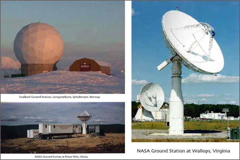
NASA ground tracking stations at
Svalbard, Wallops and Poker Flats
Usually, we scheduled a ground pass at one of the four ground stations every six hours or so. We talked to TDRSS about six times per day. Communications must be scheduled and arranged, and like all international calls, these communications passes are not cheap! Interspatial (satellite-to-satellite) calls are most expensive, and ground-to-space calls are slightly less costly. We could have talked to TDRSS and the ground stations more often, but it would have cost more money, so we generally followed our regular schedule, unless there was an emergency. During safemodes or other anomalies, we scheduled extra TDRSS and ground passes as needed. We were not in contact with the spacecraft at all times.
While streaming 32K SSR data to the ground, we cannot record to the SSR. Our data collected by the sensors during the transmission were therefore enfolded into the transmission, bypassing the SSR. Also, it was necessary to change antennas (switching from forward to aft antenna) midway through each ground pass. During these antenna changes, we lost about 30 seconds of the real-time data because it was “beamed into space”. Our overall data capture rate for the entire mission was 99.6%, significantly exceeding the 90% data capture specification in our contract with NASA. Thus, we did just fine in terms of data capture, despite the data losses during antenna switches and anomalous events. On average, it took about 12 minutes to download the entire contents of the SSR.
Relaying Data to the Stanford Mission Operations Center
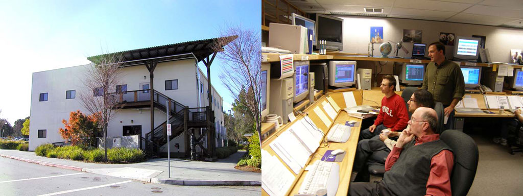
Outside and insiide the GP-B Mission
Operations Center (MOC) ~2005
When the spacecraft data were sent through TDRSS, they were then transmitted directly to the Stanford University GP-B MOC through our data link with NASA, in real time. We recorded the data on our computers in a format similar to the ground station data, and then processed it in our data processing center at Stanford. However, data relayed though ground stations went through an intermediate step, before being sent to our Mission Operations Center. When data arrives at a ground station, 32 byte headers are put on each data packet to identify it. The identifiers include our spacecraft ID, the ground receipt time, whether or not Reed-Solomon encoding was successfully navigated, the ground station ID, and several error correction checks. The data were stored at the local station and a copy was sent to a central NASA station. After it passed transmission error checks at NASA, it came to us at Stanford. The average 15-hour file took between 1.5 and 4 hours to arrive here.
Uncompressing & Formatting the Data
Once the data were received here at Stanford, a laborious process began. Spacecraft data, by its very nature, must be highly compressed so that as much data as possible can be stored. While we have over 9,000 monitors onboard, we cannot sample and store more than about 5,500 of them at a time. That’s why our telemetry is “programmable”—we could choose what data we wanted to beam down. However, in order to get as much data as possible, we compressed it highly.
The data were stored in binary format, and the format included several complexities and codes to indicate the states of more complex monitors. For example, we might encode the following logic in the data: “if bit A=0, then interpret bits B and C in a certain way; but if bit A=1, then use a very different filter with bits B and C.” The data were replete with this kind of logic. In order to decompress and decode all of this logic, we used a complex map. Our software first separated the data into its five types (described above). Then, type one underwent “decommutation.” Once all of the data in a set was translated into standard text format and decommutated, that set was stored in our vast database (over one terabyte). This was the data in its most useful, but still “raw” form; we called this “Level 1 data.” It took about an hour to process 12 hours of spacecraft data. It was the Data Processing team’s job to monitor this process, making sure files arrived intact, and unraveling any data snarls that may have come from ground pass issues.
Our science team took the Level 1 data sets, filtered them, and factored in ephemeris information and other interesting daily information (solar activity, etc). The science team also performed several important “preprocessing” steps on the data sets. Once that initial science process was complete, a data set was stored in the “Level 2” database. From there, more sophisticated analysis could be performed.
Detecting and Correcting Computer Memory Errors in Orbit

One of the Gyro Suspension System
(GSS) computers
One of the SQUID Readout Electronics
(SRE) computers
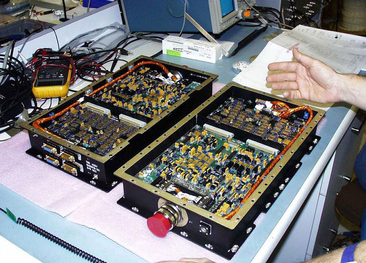
Telescope Readout Electronics (TRE)
computers
The computer and electronics systems on-board every spacecraft must undergo special “ruggedization” preparations to ensure that they will function properly in the harsh environment of outer space. GP-B's onboard computers and other electronics systems are no exception. For example, the components must be radiation-hardened and housed in heavy-duty aluminum or equivalent cases. Furthermore, the firmware (built-in hardware-level programming) must include error detection and correction processes that enable the electronic components to recover from the effects of solar radiation bombardment and other space hazards. Following is a brief description of GP-B's on-board computers and the techniques used to detect and correct single and multi-bit errors.
The Computers On-board the Spacecraft
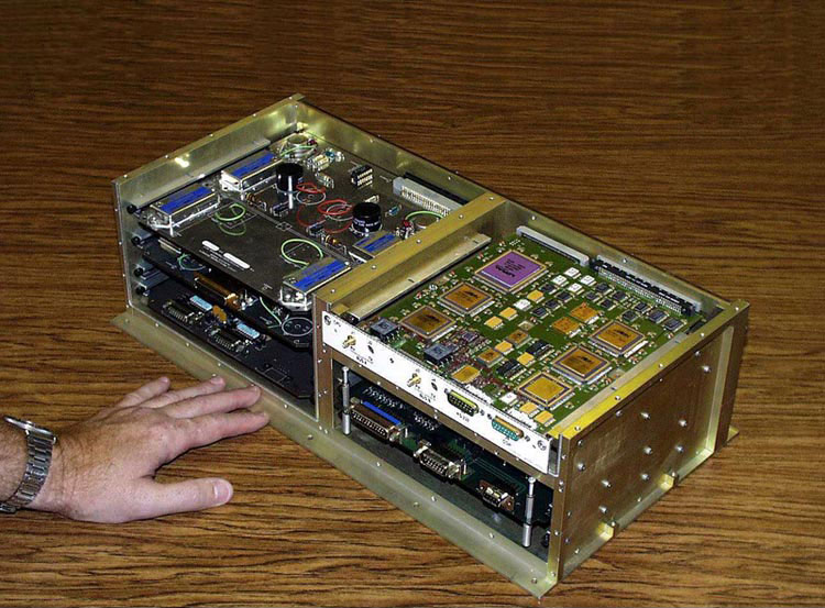
GP-B has several computers on-board the spacecraft. The main flight computer and its twin backup are called the CCCA (Command & Control Computer Assembly). These computers were assembled for GP-B by the Southwest Research Institute. They use approximately 10-year old IBM RS6000 Central Processing Units (CPUs), with 4 MB of radiation-hardened RAM memory. These computers, along with ruggedized power supplies are encased in sturdy aluminum boxes, with sides up to 1/4” thick.
In addition to the A-side (main) and B-Side (backup) flight computers, the GP-B spacecraft has two other special-purpose computers—one for the Gyro Suspension System (GSS) and one for the SQUID Readout Electronics (SRE). Each of these specialized computers contains 3 MB of radiation-hardened RAM memory and custom circuit boards designed and built here at Stanford University. Because of the custom circuit boards, these computers are housed in special aluminum boxes that were also built at Stanford.
Memory Error Detection and Correction
The RAM memory in these computers is protected by Error Detection and Correction logic (EDAC), built into the computer's firmware. Specifically, the type of EDAC logic used is called SECDED, which stands for “Single Error Correction, Dual Error Detection.” Here's how it works: For every 64 bits of RAM in the computer's memory, another 8 bits are reserved for EDAC. This produces a unique 64-bit checksum value for each RAM location. A firmware process called memory scrubbing runs continually in the background, validating the checksums for the entire bank of RAM memory locations every 2.5 seconds.
If the EDAC detects an error in which only one single bit is incorrect—a single-bit error (SBE)—in a memory location checksum value, it sends an interrupt signal to the CPU, and the CPU automatically fixes the error by writing the correct value back into that memory location. However, if the EDAC detects an error involving more than one bit—a multi-bit error (MBE)—-it generates a different type of interrupt signal causing the CPU to store the address of the bad memory location in a table that is transmitted to our mission operations center (MOC) during each telemetry communications pass.
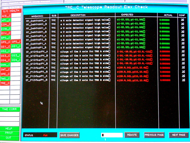
Correcting Multi-Bit Errors
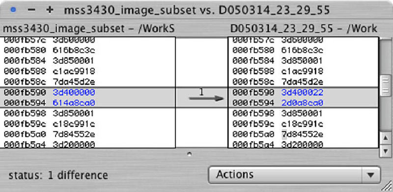
Computer screen shot showing an
example of a multi-bit error
Whenever the computer engineers on our operations team discovered the presence of one or more MBEs, they immediately looked up the use of that memory location in a map of the computer's memory. If that location was in an area of memory that was not being used, the MBE was said to have been “benign.” In fact, most, but not all, of the MBEs we experienced during the mission occurred in benign memory locations. In these cases, one of the computer engineers traveled to the Integrated Test Facility (ITF),—then located at Lockheed Martin Corporation's Palo Alto office, about 15 minutes away from the GP-B MOC, but now located at Stanford—to determine what value was supposed to be contained in the corrupted memory location. The ITF is a very sophisticated flight simulator that maintains a ground-based replica of all the systems running on the spacecraft.
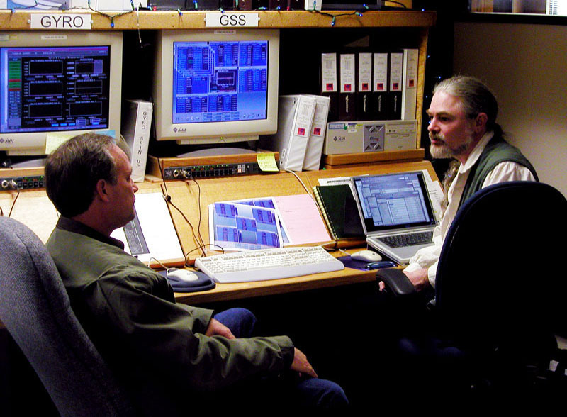
Two engineers discuss an anomaly
in the MOC.
Once the engineer determined the correct value of a bad memory location in the spacecraft's computer, he created a set of commands that were manually sent to the spacecraft during a telemetry pass to patch the bad location with the correct value. The figure to the right shows a screen capture from the ITF comparing the correct and incorrect values for a memory location from the spacecraft's computer.
On the other hand, if the engineer determined that the MBE was located in an active part of the computer's memory—a location containing a command that the CPU would be executing—he would ask the mission operations team to manually issue a command to the flight computer, stopping the timeline of instructions that was being executed, until the bad memory location could be patched. However, it turns out that there was one scenario in which an MBE in a critical part of memory could be missed by the EDAC system.
Watchdog Timer Errors
The 2.5 seconds that it takes the EDAC to scrub the entire memory may seem like a very short time in human terms, but an RS6000 CPU can execute a great many instructions in that time frame. Because the CPU is executing instructions while EDAC memory scrubbing is in process, it is possible for the CPU to access a memory location that was, say, struck by a stray proton from the sun near the SAA region of the Earth, before the EDAC system detected the error. And, if that memory location contains a corrupted instruction that the CPU tries to execute, it can cause the CPU to hang or crash. Communications hardware in the interface box connected to the computer includes a so-called “watchdog timer.” This is basically a failsafe mechanism that, like the deadman switch on a bullet train, awaits a signal from the CPU at regular intervals. If the watchdog timer expires without receiving a signal, it automatically triggers a reboot of the computer.
By a process of elimination, the GP-B Anomaly Review Team concluded that this is probably what happened in the backup CCCA (main computer) on-board the spacecraft on Friday, March 18, 2005. The flight computer maintains a history of completed instructions up to within one second of executing an instruction in a bad memory location. However, once the watchdog timer expires and the computer reboots, this history is lost. Thus, the occurrence of such an event can only be deduced by eliminating other possible causes.
Safemodes & Anomalies
Consider the following: GP-B is a unique, once-in-history experiment. Its payload, including the gyroscopes, SQUID readouts, telescope and other instrumentation took over four decades to develop. Once launched, the spacecraft was physically out of our hands, and typically, we only communicated with it about every two hours via scheduled telemetry passes. Thus, we entrusted the on-board flight computer (and its backup) with the task of safeguarding the moment-to-moment health and well-being of this invaluable cargo. How did the GP-B flight computer accomplish this critically important task? The answer is the safemode subsystem.
The GP-B Safemode System
There is a problem on-board....
Most autonomous spacecraft have some kind of safemode system on-board. In the case of GP-B, Safemode is an autonomous subsystem of the flight software in the GP-B spacecraft's on-board flight computers. The GP-B Safemode Subsystem is comprised of three parts:
- Safemode Tests—Automatic checks for anomalies in hardware and software data.
- Safemode Masks—Scheme for linking each safemode test with one or more safemode response sequences.
- Safemode Responses—Pre-programmed command sequences that are activated automatically when a corresponding test fails to provide an expected result.
These tests and response commands are designed to safeguard various instruments and subsystems on the spacecraft and to automatically place those systems in a known and stable configuration when unexpected events occur. For example, one of the tests in the GP-B Safemode Subsystem checks to ensure that the communications link between the on-board flight computer and the GP-B MOC here at Stanford is alive and active. The requirement for this test is that the flight computer must receive some command from the MOC at least once every 12 hours. If the flight computer does not receive a command within that time frame, we assume that normal telemetry is not working, and the pre-programmed response commands cause the computer to automatically reboot itself and then re-establish communication. This test is a variation of the “deadman switch” test used on high-speed bullet trains. To ensure that the train's engineer is alive and awake while the train is traveling at high speed, the engineer is required to press a button or switch at regular intervals. If the train does not receive the expected human input within each time interval, the train automatically throttles down and comes to a halt.
Not all of the tests and responses in the GP-B Safemode Subsystem were enabled at any given time. For example, some of the tests were specifically created for use during the launch and/or during the Initialization and Orbit Checkout (IOC) phase and were no longer needed during the science phase of the mission. Also, active tests and responses could be re-programmed if necessary. For example, the response commands for the safemode that triggered a computer reboot on Monday, March 14, 2005, were changed in the ensuing days to simply stop the mission timeline, rather than rebooting the flight computer, as originally programmed.
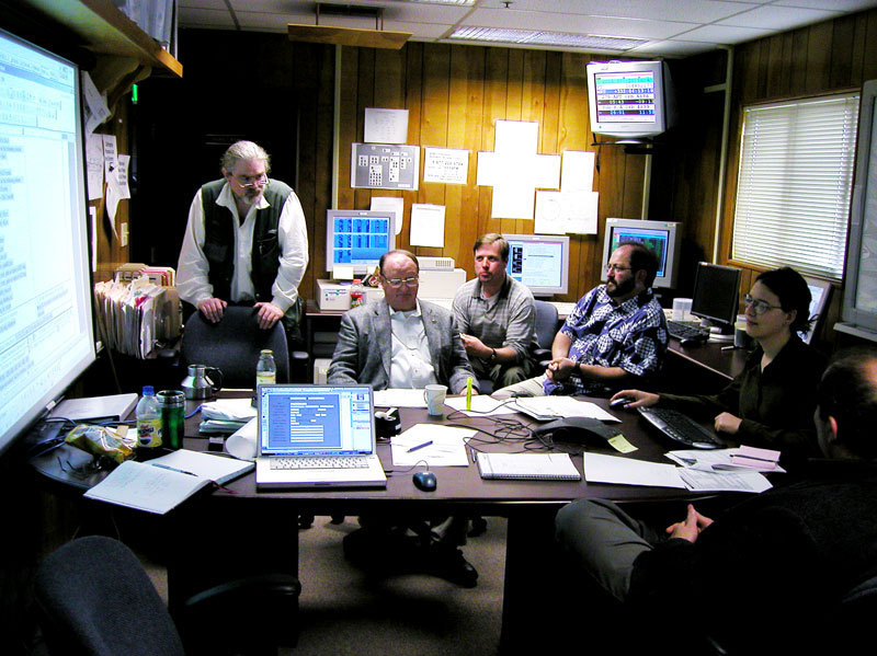
Responding to Anomalies On Orbit
Anomaly resolution in the
GP-B Mission Ops Center
When anomalous events occurred, automatic responses ensured that the spacecraft and its subsystems remained in a safe and stable condition. This enabled our mission operations team to become aware of the issue on-board, identify and understand the root cause, and take appropriate action to restore normal operations. GP-B employed a formal process, called “anomaly resolution,” for dealing with unexpected situations that occurred in orbit. This process was thoroughly tested and honed during a series of seven pre-flight simulations over the course of two years.
GP-B anomalous events were evaluated and classified into one of four categories:
- Major Space Vehicle Anomalies—Anomalies that endangered the safety of the spacecraft and/or the payload. Response to these anomalies was time-critical.
- Medium Space Vehicle Anomalies—Anomalies that did not endanger the safety of the space vehicle but could have impacted the execution of the planned timeline. Response to these anomalies was not timecritical if addressed within a 72-hour window.
- Minor Space Vehicle Anomalies—Anomalies that did not endanger the safety of the space vehicle. These were low risk problems with the vehicle that were resolved by taking the appropriate corrective action.
- Observations—In addition to formal anomaly categories, the space vehicle often exhibited off-nominal or unexpected behavior that did not appear initially to be an operational or functional issue and did not violate any limits, but warranted attention over time. Observation items were sometimes elevated to an anomaly category if they were judged to be serious enough to warrant a high-priority investigation.
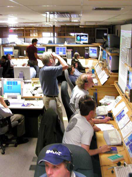
An anomaly resolution team in
action in the GP-B Anomaly Room
The GP-B Safemode Subsystem and anomaly resolution process worked very well throughout the mission. Over the course of the flight mission, the ARB successfully worked through 193 anomalies/observations. Most of these issues (88%) were classified as observations, and about 9% were classified as minor to medium anomalies. But five (3%) were classified as major anomalies, including the B-Side computer switch-over and the stuck-open valve problems with two of the 16 micro thrusters early in the mission, as well as subsequent computer and subsystem reboot problems due to solar radiation strikes. In each case, the established anomaly resolution process enabled the team to identify the root causes and provide successful recovery procedures in every case. You can read a more detailed description of the GP-B Anomaly Resolution Process in the Mission Operations section. Also, Appendix D, Summary Table of Flight Anomalies of the GP-B Post Flight Analysis—Final Report to NASA contains a table summarizing the complete set of anomalies and observations from launch through the end of the post-science calibrations in October 2005.
Effects of Anomalies on the Experimental Results
Whenever anomalous events occurred on-board the GP-B spacecraft in orbit, such as computer switch-overs and reboots, we received numerous inquiries asking about the effects of these events on the outcome of the GP-B experiment. These events have resulted in a small loss of science data. In and of itself, this loss of data will have no significant effect on the results of the experiment. If it turns out that some of the lost data was accompanied by non-relativistic torques on the gyros (measurable drift in the gyro spin axes caused by forces other than relativity), we believe that there will probably be a perceptible, but still insignificant effect on the accuracy of the end results. We really will not be able to quantify the effect of these events until the full data analysis is completed early in 2007.
We had long anticipated and planned for dealing with possible lapses in the data and non-relativistic torques on the gyros during the mission. In fact, this subject was explicitly discussed in Dr. Thierry Duhamel's 1984 PhD thesis entitled Contributions to the Error Analysis in the Relativity Gyroscope Experiment. (This was one of 85 Stanford doctoral dissertations sponsored by GP-B over the past 42 years.) Chapter 4 of Dr. Duhamel's dissertation is entitled “Effect of Interruptions in the Data.” In this chapter, Dr. Duhamel modeled various hypothetical cases of an undetermined amount of gyro spin axis drift due to non-relativistic torques (forces) on the gyros, accompanying data interruption periods of varying lengths. Each of Dr. Duhamel's hypothetical scenarios models these effects over a 12-month data collection period, showing the effect of gyro drift and data loss as a function of when in the mission (month 1, month 2, etc.) the event occurs.
In a nutshell, the results of Dr. Duhamel's research showed that lapses of data in which the gyros do not experience any non-relativistic torques would have no significant effect on the outcome of the experiment. Lapses of data that are accompanied by gyro drifts of unknown size due to non-relativistic forces would have a Gravity Probe B — Post Flight Analysis • Final Report March 2007 409 perceptible, but still relatively small effect on the experimental results. Furthermore, Dr. Duhamel's research indicates that in most cases, the effects of gyro drift and data loss tend to be larger if they occur at the beginning or end of the science phase, rather than in the middle.
Based in part on Dr. Duhamel's prescient research over 20 years ago, the GP-B science team has developed and perfected a comprehensive, state-of-the-art data analysis methodology for the GP-B experiment that, among many other things, takes into account data lapses and the possibility of accompanying non-relativistic torques on the gyros. Also, many improvements have been made in the GP-B technology since Dr. Duhamel did his research. These improvements provide us with more extensive data and extra calibrations that enable us to further refine the original error analysis predictions.
Dr. Thierry Duhamel now lives in France (his native country), where he works for EADS Astrium, a leading European aerospace company.
Aberration of Starlight—Nature's Calibrating Signal
Motion of the GP-B spacecraft over
the course of a year
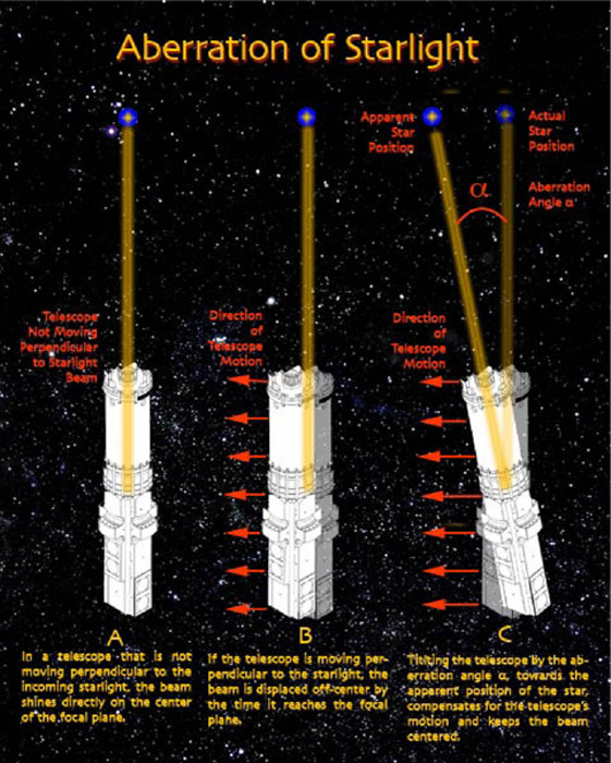
Illustration of the
aberration of
starlight
GP-B Principal Investigator, Francis Everitt, once said: “Nature is very kind and injects a calibrating signal, due to the aberration of starlight, into the GP-B data for us.” This phenomenon actually provides two natural calibration signals in the relativity data that are absolutely essential for determining the precise spin axis orientation of the gyros over the life of the experiment.
Note: You can read more about the concept of the aberration of starlight and the historical origins of this concept in our July 15, 2005 Mission News Story.
Role of Stellar Aberration in the GP-B Experiment
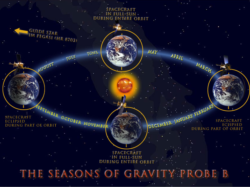
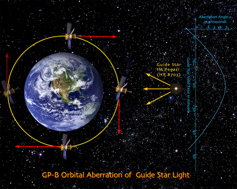
While constantly tracking the guide star, IM Pegasi, the telescope on-board the spacecraft was always in motion—both orbiting the Earth once every 97.5 minutes and along with the Earth, the spacecraft and telescope have been orbiting the Sun once a year. These motions result in two sources of aberration of the starlight from IM Pegasi. The first is an orbital aberration, which has a maximum angle of 5.1856 arcseconds, resulting from the spacecraft’s orbital speed of approximately 7 km/sec, relative to the speed of light. (In the case of orbital aberration, the relativity correction is insignificant.). The second is the annual aberration due to the Earth's orbital velocity around the Sun, which when corrected for special relativity, amounts to an angle of 20.4958 arcseconds.
In the GP-B experiment, the signals representing the precession in the gyroscope spin axes over time are represented by voltages that have undergone a number of conversions and amplifications by the time they are telemetered to Earth. These conversions and amplifications imparted a scale factor of unknown size into the data, and early on in the development of the GP-B experimental concept it was apparent that there needed to be a means of determining the size of this gyro scale factor in order to see the true relativity signal. Initially, it seemed that aberration of starlight was going to be a source of experimental error bundled into the scale factor. But upon examining this issue more closely, it became clear that, quite to the contrary, the orbital and annual aberration of light from the guide star actually provided two built-in calibration signals that would enable the gyro scale factor to be calculated with great accuracy.
The Orbital Aberration Signal
Orbital aberration of starlight
calibrating signal
To see how this works, let's first take a closer look at how the orbital aberration of the starlight from the guide star, IM Pegasi, is “seen” by GP-B spacecraft. As mentioned earlier, the spacecraft orbits the Earth once every 97.5 minutes. During the mission, as the spacecraft emerged over the North Pole, the guide star came into the field of view of the science telescope, and the telescope then locked onto the guide star. This began what was called the “Guide Star Valid (GSV)” phase of the orbit. At this point in its orbit, the orientation of the spacecraft's velocity was directly towards the guide star, and thus, there was no aberration of the star's light—it traveled straight down the center of the telescope. However, as the spacecraft moved down in front of the Earth, the orientation of its velocity shifted in the orbital direction until it became perpendicular to the direction of the light from the guide star, slightly above the equator. This is the point of maximum aberration since the telescope was then moving perpendicular to the guide star’s light. As the spacecraft moved on towards the South Pole and then behind the Earth and directly away from the guide star, the aberration receded back to zero. At this point, the telescope unlocked from the guide star, transitioning into what was called the “Guide Star Invalid (GSI)” phase of the orbit. The navigational rate gyros on the outside of the spacecraft maintained the telescope's orientation towards the guide star while the spacecraft was behind the Earth, but we did not use the science gyro data collected during the GSI phase.
During the GSV portion of each orbit, the telescope remained locked on the guide star, with the spacecraft's micro thrusters adjusting the telescope's pointing for the aberration of the guide star's light. This introduced a very distinct, half-sine wave pattern into the telescope orientation. This sinusoidal motion was also detected by the gyro pickup loops that are located in the gyro housings, along the main axis of the spacecraft and telescope. Thus, this very characteristic pattern, generated by the telescope and thrusters, appeared as a calibration signal in the SQUID Readout Electronics (SRE) data for each gyro.
The Annual Aberration Signal

Annual aberration of starlight
calibrating signal
The annual aberration of the guide star's light works the same way as the orbital aberration signal, but it takes an entire year to generate one complete sine wave. Using the spacecraft's GPS system, we can determine the orbital velocity of the spacecraft to an accuracy of better than one part in 100,000 (0.00001). Likewise, using Earth ephemeris data from the Jet Propulsion Lab in Pasadena, CA, we can determine Earth's orbital velocity to equal or better accuracy. We then used these velocities to calculate the orbital and annual aberration values with extremely high precision, and in turn, we used these very precise aberration values to calibrate each of the gyro pointing signals. It is interesting to note that the amplitude of the sine wave generated by the annual aberration is four times as large as the orbital aberration amplitude, with peaks occurring in September and March. Because we launched GP-B in April and started collecting science data in September, the effect of the annual calibration signal did not become apparent in the data until February-March 2005, six to seven months into the science phase of the mission. Thus, from March 2005 - August 2005, both the annual and orbital aberration signals were used in the ongoing analysis of the science data.
Telescope Dither—Correlating the Gyroscope & Telescope Scale Factors
When used in reference to technology, the term, dither, generally refers to the seemingly paradoxical concept of intentionally adding noise to a system in order to reduce its noise. For example, a random dithering technique is used to produce more natural sounding digital audio, and another form of visual dithering enables thousands of color shades, used on Internet Web sites, to be derived from a limited basic palette of 256 colors. With respect to the GP-B spacecraft, the dither refers to an oscillating movement of the science telescope and spacecraft that was activated whenever the telescope was locked onto the guide star. This intentional telescope movement produced a calibration signal that enabled us to relate the signals generated by the telescope photon detectors to the signals generated by the SQUID magnetometer readouts of the gyro spin axis positions.
The Science Telescope—Centering on the Guide Star
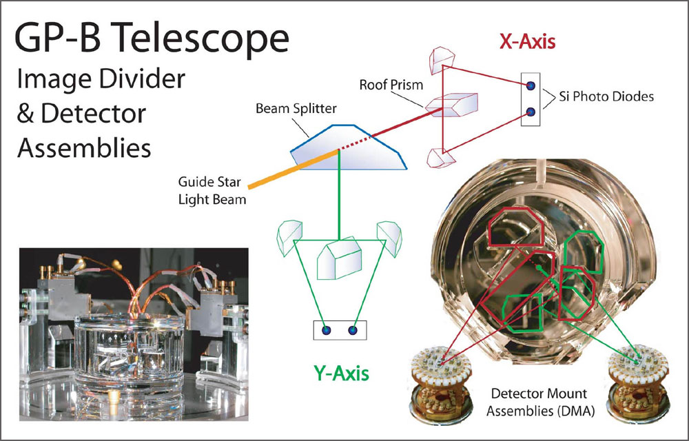
Diagram of the science telescope
image divider and detectors
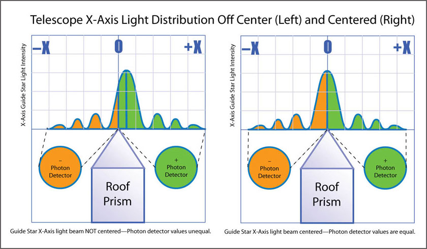
The sole purpose of the GP-B science telescope was to keep the spacecraft pointed directly at the guide star during the “guide-star-valid” portion of each orbit—that is, the portion of each orbit when spacecraft was “in front of ” the Earth relative to the guide star and the guide star was visible to the telescope. This provided a reference orientation against which the spin axis drift of the science gyros could be measured. The telescope accomplished this task by using lenses, mirrors, and a half-silvered mirror to focus and split the incoming light beam from the guide star into an X-axis beam and a Y-axis beam. Each of these beams was then divided in half by a knife-edged “roof ” prism, and the two halves of each beam were subsequently focused onto a pair of photon detectors. When the detector values of both halves of the X-axis beam were equal, we knew that the telescope was centered in the X direction, and likewise, when the detector values of both halves of the Y-axis beam were equal, the telescope was centered in the Y-axis direction. (The telescope actually contains two sets of photon detectors, a primary set and a backup set for both axes.)
Normalized Pointing
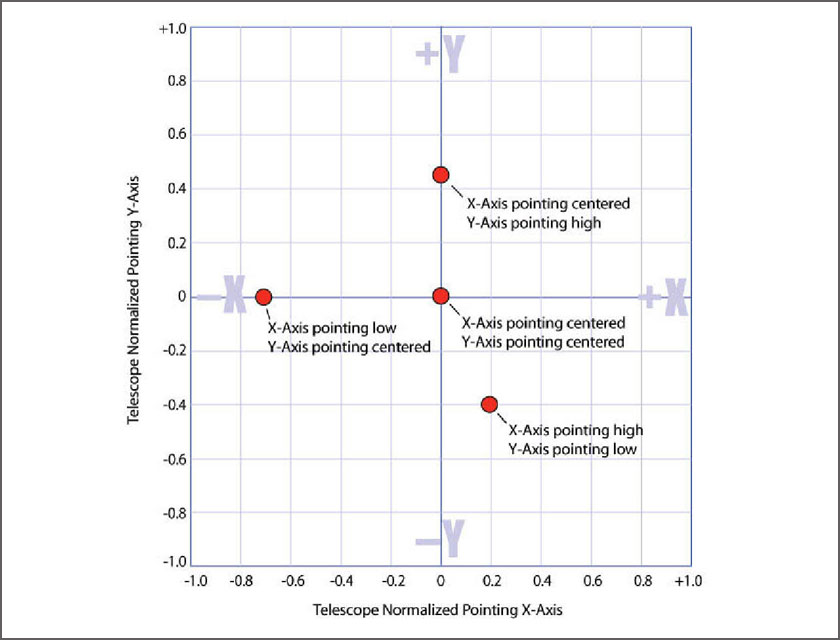
Normalizing (mapping) telescope readout
signals onto a range from -1 to +1
Comparing detector signals to center
the telescope on the guide star

Illlustration of the science telescope
dither pattern
The telescope detector signals were converted from analog to digital values by the Telescope Readout Electronics (TRE) box, and these digital values were normalized (mapped) onto a range of -1 to +1. In this normalized range, a value of 0 meant that the telescope was centered for the given axis, whereas a value of +1 indicated that all of the light was falling on one of the detectors and a value of -1 indicated that all of the light was falling on the other detector.
In actuality, the light beam for each axis was distributed in a bell-shaped curve along this scale. When the telescope was centered, the peak of the bell curve was located over the 0 point, indicating that half the light was falling on each detector. If the telescope moved off center, the entire curve shifted towards the +1 or -1 direction. You can think of this as a teeter-totter of light values, with the 0 value indicating that the light was balanced, as shown in the middle figure to the right..
The Telescope Dither Pattern
A telescope scale factor translated the values on this normalized scale into a positive or negative angular displacement from the center or 0 point, measured in milliarcseconds (1/3,600,000 or 0.0000003 degrees). Likewise, a gyro scale factor translated converted digital voltage signals representing the X-axis and Y-axis orientations of the four science gyros into angular displacements, also measured in milliarcseconds. We then had both the telescope and gyro scale factors defined in comparable units of angular displacement. The telescope dither motion was then used to correlate these two sets of X-axis and Y-axis scale factors with each other. The telescope dither caused the telescope (and the entire spacecraft) to oscillate back and forth in both the X and Y directions around the center of the guide star by a known amount.
Because this motion moved the entire spacecraft, including the gyro housings that contain the SQUID pickup loops, the SQUIDs detected this oscillation as a spirograph-like (multi-pointed star) pattern that defined a small circle around the center of the guide star. This known dither pattern enabled us to directly correlate the gyro spin axis orientation with the telescope orientation. The result was a pair of X-axis and Y-axis scale factors that were calculated for the guide-star-valid period of each orbit. At the end of the data collection period on August 15, 2005, we had stored approximately 7,000 sets of these scale factors, representing the motion of the gyro spin axes for the entire experiment.
At the beginning of May 2005, we turned off the dither motion for a day to determine what effect, if any, the dither itself was contributing to our telescope pointing noise and accuracy. The results of this test indicated that the navigational rate gyros, which were used to maintain the attitude of the spacecraft and telescope during guide-star-invalid periods (when the spacecraft was behind the Earth), were the dominant source of noise in the ATC system, whereas the science gyro signals were stronger than the noise in the SQUID Readout Electronics (SRE) system.
Isolating the Gyroscope Signals from Noise & Interference
Conceptually the GP-B experimental procedure is simple: At the beginning of the experiment, we initially pointed the science telescope on-board the spacecraft at the guide star, IM Pegasi, and we electrically nudged the spin axes of the four gyroscopes into the same alignment. Then, over the course of a just under a year, as the spacecraft orbited the Earth some 5,000 times while the Earth made one complete orbit around the Sun, the four gyros spun undisturbed—their spin axes influenced only by the relativistic warping and twisting of spacetime. We kept the telescope pointed at the guide star, and each orbit, we recorded the cumulative size and direction of the angle between the gyroscopes' spin axes and the telescope. According to the predictions of Einstein's general theory of relativity, over the course of a year, an angle of 6,606 milliarcseconds should have opened up in the plane of the spacecraft's orbit, due to the warping of spacetime by the Earth, and a smaller angle of 39 milliarcseconds should have opened up in the direction of Earth's rotation due to the Earth dragging its local spacetime around as it rotates. In reality, what went on behind the scenes in order to obtain these gyro drift angles was a very complex process of data reduction and analysis that is taking the GP-B science team more than a year to bring to completion.
GP-B Data Levels
Throughout the science phase of the GP-B mission, we continuously collected data during all scheduled telemetry passes with ground stations and communications satellites, and these telemetered data were stored— in their raw, unaltered form—in a database here at the GP-B Mission Operations Center. This raw data is called “Level 0” data. The GP-B spacecraft is capable of tracking some 10,000 individual values, but we only captured about 1/5 of that data. The Level 0 data include a myriad of status information on all spacecraft systems in addition to the science data, all packed together for efficient telemetry transmission. So, our first data reduction task was to extract all of the individual data components from the Level 0 data and store them in the database with mnemonic identifier tags. These tagged data elements were called “Level 1” data. We then ran a number of algorithmic processes on the Level I data to extract ~500 data elements to be used for science data analysis, and this was called “Level 2 data.” While Level 2 data include information collected during each entire orbit, our science team generally only uses information collected during the Guide Star Valid (GSV) portion of each orbit when the telescope was locked onto the guide star. We do not use any gyroscope or telescope data collected during the Guide Star Invalid (GSI) portion of each orbit—when the spacecraft is behind the Earth, eclipsed from a direct view of the guide star—for science data analysis.
Dealing with Gaps in the Data
Analyzing the data collected in the GP-B experiment is similar to fitting a curve to a set of data points—the more data points collected, the more accurate the curve. If there were no noise or error in our gyro readouts, and if we had known the exact calibrations of these readouts at the beginning of the experiment, then we would need only two data points—a starting point and an ending point. However, there is noise in the gyro readouts, so the exact readout calibrations had to be determined as part of the data collection and analysis process. Thus, collecting all of the data points in between enables us to determine these unknown variables. In other words, the shape of the data curve itself is just as important as the positions of the starting and ending points.
All measurements we collected were time-stamped to an accuracy 0.1 milliseconds. This enables our science team to correlate the data collected from all four gyros. If one gyro's data are not available for a particular time period, such as the first three weeks of the science phase when gyro #4 was still undergoing spin axis alignment, that gyro is simply not included in the analysis for that particular time period. In cases where all science data are lost for an orbit or two, the effect of these small data gaps on the overall experiment is very small. Examples of such data gaps include the March 4, 2005 automatic switch-over from the A-side (main) on-board computer to the B-side (backup) computer, and a few telemetry ground station problems over the course of the mission.
Sources of System Noise & Interference
Another important point is that the electronic systems on-board the spacecraft do not read out angles. Rather, they read out voltages, and by the time these voltages are telemetered to Earth and received in the science database here in the Stanford GP-B Mission Operations Center, they have undergone many conversions and amplifications. Thus, in addition to the desired signals, the GP-B science data include a certain amount of random noise, as well as various sources of interference. The random noise averages out over time and will not be an issue. Some of what appears to be regular, periodic interference in the data is actually important calibrating signals that enable us to determine the size of the scale factors that accompany the science data. In the section, Aberration of Starlight—Nature’s Calibrating Signal above, we described how the orbital and annual aberration of the starlight from IM Pegasi is used as a means of calibrating the gyro readout signals. Likewise, in the section Telescope Dither—Correlating the Gyro & Telescope Scale Factors above, we described how the telescope dither motion is used to calibrate the telescope signals. However, the science data also include other nosie and interference that are difficult to distinguish from the relativity signals. If these sources of noise and interference can be identified, understood and modeled, they can be removed from the data, thereby increasing the accuracy of the experimental results; otherwise, they contribute to the level of experimental error.
In this regard, early in the data analysis process, we discovered two unexpected complications in the data:
- Larger than expected “misalignment” torques on the gyroscopes that produced significant classical drifts
- A damped polhode oscillation that complicated the calibration of the instrument’s scale factor against the aberration of starlight
Analyzing, understanding, modelling and removing the effects of these two complications in the data has beem a painstaking process that has significantly lengthened the data analyis phase of the mission and is still in process. You can read a detailed description of these two complications in our Summer 2007 Status Update. The current GP-B Status Update describes the progress we have made since that time.
Proper Motion of IM Pegasi—The Final Data Element

Drawing of the proper motion of the
GP-B guide star, IM Pegasi
Finally, there is one more very important factor that must be addressed in calculating the final results of the GP-B experiment. We selected IM Pegasi, a star in our galaxy, as the guide star because it is both a radio source and it is visually bright enough to be tracked by the science telescope on-board the spacecraft. Like all stars in our galaxy, the position of IM Pegasi as viewed from Earth and our science telescope changes over the course of a year. Thus, the GP-B science telescope is tracking a moving star, but gyros are unaffected by the star's so called “proper motion;” their pointing reference is IM Pegasi's position at the beginning of the experiment. Thus, each orbit, we must subtract out the telescope's angle of displacement from its original guide star orientation so that the angular displacements of the gyros can be related to the telescope's initial position, rather than its current position. The annual motion of IM Pegasi with respect to a distant quasar has been measured with extreme precision over a number of years using a technique called Very Long Baseline Interferometry (VLBI) by a team at the Harvard-Smithsonian Center for Astrophysics (CfA) led by Irwin Shapiro, in collaboration with astrophysicist Norbert Bartel and others from York University in Canada and French astronomer Jean-Francois Lestrade. However, to ensure the integrity of the GP-B experiment, we added a "blind" component to the data analysis by requesting that the CfA withhold the proper motion data that will enable us to pinpoint the orbit-by-orbit position of IM Pegasi until the rest of our data analysis is complete. Therefore, the actual drift angles of the GP-B gyros will not be known until the end of the data analysis process.
Science Data Analysis Process
In this section we first provide a brief overview of what is involved in analyzing the GP-B science data. Data analysis actually began before launch. The science data analysis team built prototype computer codes to process simulated science data in preparation for the actual data from the spacecraft. Following on-orbit checkout, the team used real data to test and refine these routines and to take into account the anomalies the mission has encountered (i.e. the time varying polhode period) that were not part of the initial simulations. These activities all preceded the formal data analysis effort.
Three Data Analysis Phases
Following acquisition and archiving of the science data from the satellite, the formal analysis of these data is broken into three phases; each subsequent phase builds upon the prior toward the final science results.
- Phase 1: Short-term (day-by-day) analysis—Initially, the data are analyzed primarily over a short time period, typically a few orbits or a day, with the goal to understand the limitations of data analysis routines and to improve them where necessary. The major activities of this phase include:
- Final instrument calibrations are completed, based on the IOC, the Science Mission, and the Post- Science Calibration tests run on the vehicle.
- Refinements are made to the subsystem performance estimates (i.e. GSS, ATC, TRE, SRE subsystems). The performance of these systems sets lower bounds on the quality of the results we expect to obtain from the experiment.
- Through the data analysis, known features are removed—for example, aberration and pointing errors were removed from the science signals.
- A data grading scheme is implemented to flag and optionally ignore patches of the data set that are not of science quality due to spacecraft anomalies or off-nominal configuration of the instrument.
- Phase 2: Medium-term (Month-to-month) analysis—In this second phase, the analysis team’s attention turns to understanding and compensating for long-term systematic effects that span many days or months, such as those that arise from the time-varying gyro polhode period or drifts in the calibrations of the on-board instrumentation.
- Identify, model, and remove systematic errors and improve instrument calibrations.
- Understand causes and implications of spacecraft anomalies. Model and remove effects resulting from these anomalies.
- Assess the magnitude of residual Newtonian torques on the gyroscopes and compare with pre-launch estimates.
- Phase 3: One-Year perspective—In the final phase, the data from all four gyroscopes are combined with the guide star proper motion measurements, provided by our partners at the Smithsonian Astrophysical Observatory (SAO), to generate an overall estimate of the gyroscope precession rates over the mission. These estimates form the basis of the primary science result: the precession of the gyroscopes due to the effects of general relativity. This process will naturally produce a third, improved, “orientation of the day” for each of the gyroscopes.
The overall goals of this phase are to improve the quality of the science data analysis package, calibrate out instrumentation effects, and produce an initial “orientation of the day” estimate based on the tuned-up data analysis package. It does not attempt at this stage to remove systematic errors that span many days or months. In addition, this analysis focuses on each gyros’ performance individually and does not attempt to combine the four measurements, and it does not attempt to estimate the gyroscope precession (due to either relativistic or classical effects)
The primary products from this phase are a “trend of the month” per gyroscope, which is the initial estimate of the measured gyroscope precession over a medium time scale (approximately 1 month) after the compensation of identified systematic error sources. This phase will also produce a refined “orientation of the day” per gyroscope. Here, too, the focus is on individual gyroscope performance.
Independent Data Analysis Teams
The Stanford team has formed two independent, internal teams to attack the data analysis task. This was done primarily for internal quality control: two teams, processing the exact same data, should produce very similar results. The results are compared formally on a regular basis where discrepancies are noted and investigated. These comparisons will unearth subtle software coding errors, which may go undetected if only a single analysis package is used. Each team, while working under the constraint of using the same source data, has considerable latitude in what methods of analysis to apply during each of the data analysis phases. This has the beneficial effect of better understanding the nature of the source data and what signal processing techniques are most effective in estimating the performance of the four science gyroscopes.
To provide a benchmark for both of the teams, sets of “truth model data” are constructed and are run on the two data analysis packages. In these truth model cases, the signal structure, instrument calibrations, and noises are precisely known and can be analyzed in a relatively straightforward way without sophisticated signal processing tools. Both data analysis packages should return identical results when run on such truth data; if they do not, this test reveals a fundamental difference in the algorithms that may be rectified quickly. Once the algorithms agree on “truth”, they will be re-benchmarked regularly to ensure that evolutionary changes in the codes do not compromise their ability to correctly analyze straightforward data sets.
Data Grading
The Gravity Probe B science data consists of approximately 5300 guide star valid intervals during which the instrument is able to measure the orientation of each of the four gyroscopes with respect to the line of sight to the guide star. Due to vehicle anomalies or environmental effects, not all of these intervals contain valid science measurement data. If these data are used in the analysis algorithms, significant errors in the overall results may be introduced.
Consequently, a data grading scheme is used to separate the compromised data from the clean science data. The grading system does not remove data from the set, but simply flags segments of the data that do not meet an established grading criteria. Roughly 20 criteria have been set to flag sub-standard data on a gyro-by-gyro basis. The criteria chosen are primarily a function of vehicle state, such as “guide star out of view,” “vehicle in eclipse”, “loss of drag-free control,” “SQUID unlocked;” these all directly affect the validity of the data being sent from the spin axis readout system.
During data analysis runs, the analyst selects the grading criteria that will apply during the run. Then, database extraction tools will then return the data that meet the grading criteria. Immediately, the same algorithm can be run with different grading criteria to assess the sensitivity of the result to various types of low quality data.
The Data Analysis "Standard Model"
The GP-B data analysis "Standard
Model"
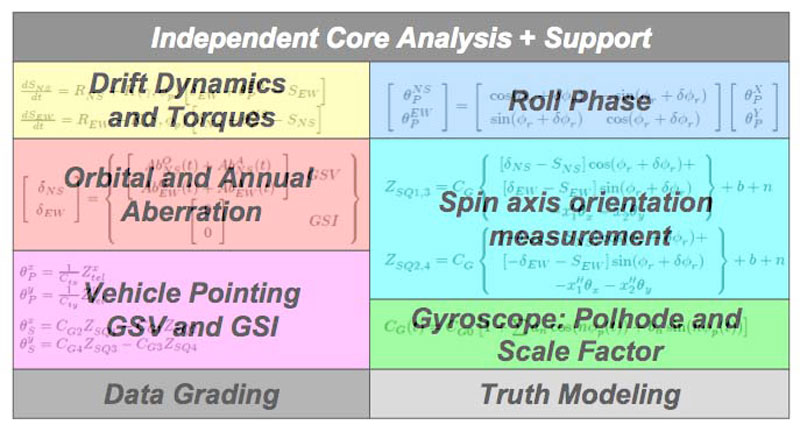
The data analysis effort revolves around a “standard model” for how the vehicle operates and how vehicle configuration affects the performance of the gyroscopes. This model evolves as the team’s knowledge of the operation and performance of the vehicle increases during the analysis efforts. In addition to the 1) Independent Analysis teams, 2) the Truth Modeling Efforts, and 3) the Data Grading system, the data analysis team focuses its efforts on six primary areas of vehicle performance:
- Precession dynamics and torques: Understand the overall drift of the gyroscope and how it relates to relativistic effects and classical (Newtonian) effects.
- Orbital and Annual Aberration: Model and compensate for the apparent motion of the guide star due to space vehicle motion.
- Vehicle Pointing: Assess the pointing of the space vehicle during guide star valid (GSV) and guide star invalid (GSI) periods using all on-board sensors (ATC, telescope, science gyroscopes). Determine relative scale factor between telescope readout of pointing and science gyroscope readout of pointing.
- Roll Phase Measurement: Measure and quantify errors in the roll phase of the vehicle over the mission (time history of the clocking of the vehicle with respect to the orbital plane).
- Spin Axis Orientation Measurement: Model and calibrate the SQUID readout system and compensate for effects of vehicle pointing in the science signal.
- Polhode and Scale Factor Modeling: Model and remove the effects of the time varying polhode period on the SQUID scale factor. Compensate for systematic errors in gyro orientation measurements due to the slow damping of the gyroscope polhode path.
Phase 1 activities focus primarily on improving the accuracy of all the terms that go into the standard model, based on vehicle data, and setting performance limits on the ultimate resolution of the experiment. Phase 2 and 3 activities focus on the precession dynamics, effects of anomalies, and polhode models that span weekly or monthly time scales. Though only shown in a simple outline here, the standard model gives a convenient frame of reference for the whole team in which to discuss results and propose new explanations and models for observed phenomena.
Publication of Final Results
Based on the successful results announcement strategies for the COBE and WMAP missions, the Gravity Probe B project will announce the results of the experiment only after the internal data analysis effort is complete (Phases 1, 2, and 3, above), and after critical and detailed peer review of the results from the gravitational physics community. No data or preliminary results will be released prior to this point. This is done to insure the integrity of the result and maintain credibility within the wider scientific community. Once this work is complete and both the internal and external review teams are satisfied with their reviews, the results will be presented, along with a coordinated set of papers on the design and operation of the mission, at a major physics conference. You can follow our GP-B science team's progress in the data analysis process in the Status section of this Web site.
<- Mission Operations (Previous) | Legacy (Next) ->